Measuring Frequency Response

by Tim Wescott, Wescott Design Services

(note: For more information on measuring and interpreting a system's frequency response, and other practical uses of control theory, see the book Applied Control Theory for Embedded Systems.)

0.1

1 Overview

When you design a control system using any of the frequency response methods � Bode plot, Nyquist plot or Nichols chart � it is not necessary to refer to the z-domain transfer function of the plant or controller except to find the system gain and phase response over the frequency range of interest. It is possible, therefore, to use a set of frequency response data without having an exact z-domain transfer function in hand. Furthermore, the frequency response data doesn't need to come from a mathematical model of the system � it can just as well come from a set of measured frequency responses. This means that you can do a very good job of control system design without ever having a known model of your plant; it is sufficient to have a set of measured frequency responses complete enough for your design.

Knowing this, one is immediately motivated to ask �so how do I measure the frequency response?� There are measuring instruments that have been developed to do this¹, but they are expensive and in a digital control system they are difficult to integrate. For little more than the effort required to integrate a control systems analyzer into your system you can build the necessary interfaces into your software to allow you to collect and analyze the necessary data on your PC, with the added bonus that the resulting data will be in a form that you can immediately use for designing your control system.

There are a number of facets to measuring frequency response that must be addressed. You must excite the system with the correct sinusoidal waveform and you must collect the resulting system behavior and extract the relevant frequency response data from it. This must be done in a manner that is relatively immune from the noise than inevitably permeates a real-world control system, that is practical, easy to use, and doesn't add significantly to the cost of your system.

2 Measuring In Isolation

The most direct way to measure a system's response at a given frequency is accomplished by driving the system under test with a sine wave at the desired frequency while monitoring the relevant system output(s). Then find the amplitude and phase of the response, and compare this amplitude and phase to the amplitude and phase of the injected sine wave. To find a complete system frequency response over some span, you excite the system with a sine wave, taking a set of measurements at a frequency, stepping the frequency up (or down) and repeating as necessary until the desired data set has been collected.

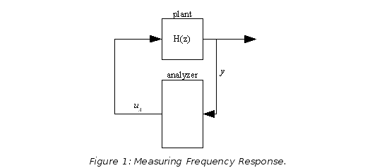
Take the setup shown in Figure 1, where the goal is to find the frequency response of the plant who's transfer function is H(z). For any given frequency f (in cycles per sample) we set the input signal

where k is the sample index and A_T is chosen to keep from overloading the plant. Assuming that the plant is stable and linear the output of the plant will be of the form

where A(f) and φ(f) are the gain and phase of the frequency response at f and y_T(k) is a transient signal which will go to zero as k goes to infinity.

To actually find the values of A(f) and φ(f) you can measure the response over some finite number of samples and compute the first term of the Fourier series for y(k):

and

where (5) arc tangent takes the �four quadrant� arc tangent. The equations in (3) only work well if the samples are taken over an integer number of cycles of the input, i.e. if N is an integer multiple of 1/f, and they work best if the transient signal is reduced as much as possible � it is usually helpful to start from zero with a sine wave and to have a delay before the data is collected or to follow data collection at one frequency with data collection at a close-by frequency.

If you recall Euler's identity,

(3) and (4) become

where the ­π/2 term on the right-hand side compensates for the fact that the excitation is a sine wave rather than a cosine wave. This is a handy relationship to remember if you are using a math package to do your computation, as you can reduce (6) down to a single vector multiply with very efficient computation with such a package.

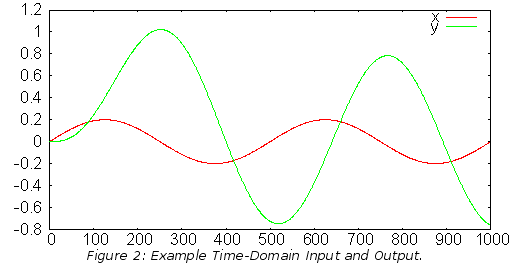
For example Figure 2 shows the response of a 2^nd-order system at a frequency of f = 1/500. There is an initial turn-on transient, but the system is already settling out by the end of two cycles. If we apply (3) to the entire data sample in Figure 2 we see an error of about 20% from the actual transfer function, but applying it to the last 500 samples gives us an error under 3%.

Normally you are going to be interested in making measurements at a number of frequencies that will be fairly closely spaced. In this case the best way to reduce the startup transient is just to insure that the input sinusoid changes smoothly � as long as it does not stop or exhibit phase jums at the frequency boundaries then the transients will be negligible for most systems.

3 In-Loop Measurement

The setup in Figure 1 and equation (3) are sufficient for taking measurements of a well-behaved system in isolation. If, however, you are interested in more than just the behavior of one system (or subsystem) taken in isolation, if you want to know how your system behaves in closed loop, or if you are dealing with an unruly or unstable plant or other subsystem, it falls short.

What you need in such a case is a setup and analysis method that lets you measure the frequency response of a portion of a working system without significantly rearranging the system structure � specifically without opening up any working control loops.

What we need is a setup that will allow us to measure the frequency response of a portion of the system without opening the control loop. To do this we note that the transfer function of a block is the ratio of its input to its output. In the discussion so far we've excited a block with a sine wave and extracted its output � but in the process of extracting the output parameters in (9) we divided by the first Fourier term of the sine wave excitation, i.e. j A_T. If we choose our block, insure that it has sinusoidal input and output at our desired frequency, then measure both its input and its output and divide their first Fourier term outputs then you'll have the blocks gain and phase at the frequency in question.

Taken from a purely signal-flow perspective the setup to measure frequency response is straightforward: place a summing junction in your system at a convenient location, then monitor the signals that sit at the input and output to the section of the system who's response you want to measure. The summing junction allows us to inject a sine wave which will then pervade the entire system, while the two outputs will let us get the pair of numbers that we need to get the ratio of a block's input to output.

Figure 3 shows the signal paths for measuring the response of the plant (note that any drivers, DACs, ADCs and sampling is happening within the plant model; we're only interested in the plant behavior as seen by software). A signal, u_A is injected into the system right before the plant; the drive to the plant is picked off at the reference, u_R, and the system error is picked off at y. Assuming that the system command is held at zero this setup will measure just the plant response.

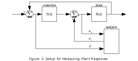
Figure 4 shows the signal paths for measuring the open-loop response of the system. Here the signal is injected in the same place, and the reference pickoff is still immediately before the drive signal, but the output pickoff is measured after the signal has passed through both plant and controller.

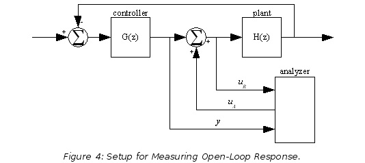
The way to extract the frequency response of the subsystem under test is the same for Figure 3 and Figure 4: inject a swept-frequency sine wave at u_A at each frequency point, apply (3) to u_R and y, and divide the two resulting numbers � the result is the frequency response at that point.

This is done with the following set of equations. First find the first Fourier coefficient for the two variables:

Then divide the resulting complex numbers to find the value of the frequency response:

For example, say we wish to measure the plant response, open-loop response and closed-loop response of a system such as the one shown in Figure 3 and Figure 4, where we're sampling at 1kHz. We don't know it, but the plant transfer function is

We do know the controller transfer function, it is

with k_d = 100, k_p = 2 and k_i = 0.01.

With a frequency sweep from 1/10^th Hz to 500Hz, we get the plant input and output, which are shown in Figure 5 and Figure 6. You can see that as the magnitude of the response gets small the signal gets noisy, as seen on the right in Figure 5 and on the left in Figure 6.

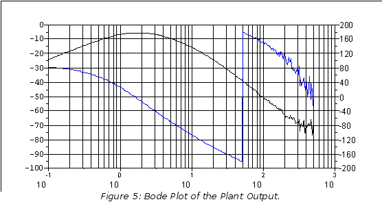
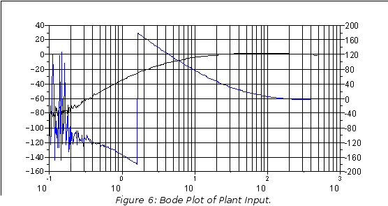
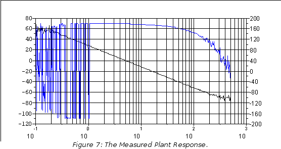
Taking these two sets of data and performing complex division on each frequency point, then plotting the results yields the response shown in Figure 7. This measured plant response can then be use with a controller model (which should certainly be exact!) to tune the system.

Rearranging the data collection to that shown in Figure 4, we measure the output of the controller and the input to the plant. The input to the plant hasn't changed, and the measured controller output is shown in Figure 8 (which is, incidentally, the closed-loop response multiplied by ­1). Dividing the controller output by the plant input gives us Figure 9.

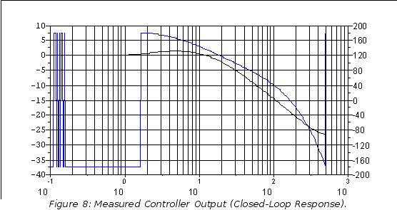
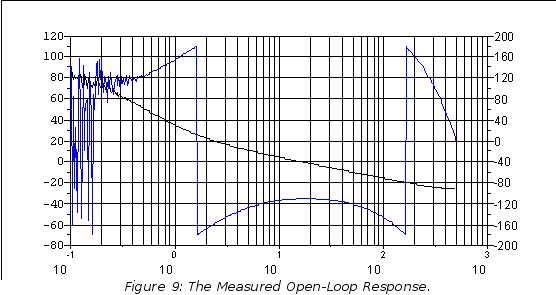
On inspecting Figure 9 it can be immediately seen that the gain-crossing frequency occurs at about 16Hz with a phase margin of about 68�, and that there are phase-crossing frequencies at 1.6Hz and 160Hz, with gain margins in excess of 20dB.

4 Real-World Issues

4.1 Noise

Noise is an inevitable part of any measurement, and in control system design it is often useful to get frequency response data over several decades of the plant response. When doing these measurements noisy data is inevitable, but as long as you understand the effects of the noise on your measurement you can mitigate them.

In Figure 7 we saw the effect of measurement noise at both ends of the spectrum. The measurement noise is constant across the frequency spectrum, but the quantities being measured varies: at the low-frequency end of the spectrum the loop gain is very high and the closed-loop gain is unity. This causes the signal at the input to the summing junction to be very small, so it can be corrupted by noise. At the high-frequency end of the spectrum the loop gain is small, so the signal level at the output of the summing junction is small and once again the measurement noise can dominate.

To mitigate the effects of noise in the measurements you must increase the signal to noise ratio in the final numbers arrived at using (3). This can be done in one of two ways: first, increase the signal by increasing the amplitude of the sine wave that you insert into your system; and second, increase the amount of time that you collect data at any particular frequency.

Increasing the signal amplitude gives the obvious advantage of more signal. You must take care, however, that you are not increasing the drive signal to the point where your system goes nonlinear through overflow or other effect (see the next section).

Increasing the amount of time over which you collect data gives you better signal to noise ratio because the operation of (3) gives a result that is coherent (i.e. synchronized) with the input sine wave, but the noise signal is incoherent. As a result the average signal amplitude rises in proportion to the length of time you collect data, but the expected amplitude of the noise only rises as the square root of this time � so increasing the collection time at each frequency by a factor of 4 will double the eventual signal to noise ratio.

4.2 Nonlinearities

Nonlinearities are an inevitable part of designing a control system, because ultimately there are no physical systems (including real software running on real processors) that don't exhibit nonlinearities. Often the nonlinearities that we must design around are slight compared to our control system requirements; in such cases it is not a bad idea to design our system using describing function analysis � and swept-sine frequency response data is exactly what is necessary for such design.

In our original analysis we justified using (3) to demodulate our data because of the form observed in (2). But (2) only follows from (1) if you assume that the system being tested is linear, or is being operated in a linear region. With a system that is not operating in a linear region (2) is not, in general, valid. In fact, the whole notion of using frequency response analysis in not generally valid for nonlinear systems.

What to do? Is this entire methodology one that only applies to that small subset of systems that is acting exactly like a linear system for the particular input that we expect? Fortunately the answer to this question is no. In the case when we are testing a stable nonlinear system then the response to a sinusoidal input is still periodic but in addition to containing energy at the fundamental frequency f it will also contain energy at DC (f = 0) 2f, 3f, etc., so (2) becomes

and A₁ (the fundamental Fourier term) is the same as A in (3). If the value of A₁ is significantly larger than any of the higher-order responses (A₂ through A_∞) then describing function analysis says that we can conveniently ignore the nonlinearities and just use the system as described by A₁(f) and φ₁(f).

Fortunately, the demodulation described in (9) or (3) will only respond to the fundamental energy in y(k), so the DC component (A₀) and all of the higher-order terms in the summation evaluate to zero. What comes out of these demodulation operations are the amplitude and phase information for the fundamental frequency only � which is usually exactly what you want in describing function analysis.

But how can you tell if the system you are measuring is operating in its nonlinear region, and how can you quantify �how nonlinear� it is? The three methods that you can use are: One, look at your system's behavior to see if an output, input, or intermediate value is hitting a maximum limit during operation; two, repeat sweeps with different input amplitudes and compare their results and three, use measures of data correlation.

Observing your system behavior is probably the best way to insure that the system is operating in its linear region if you have a good idea of how your system works. Examples of things to look for are: the system drive to see flat-topping on its output, the mechanisms themselves to see if it is hitting any stops, the system sensors to see if they are saturating even when the thing they are measuring isn't, and finally making sure that no signals are so small that they are falling into the cracks of gear train backlash or ADC/DAC precision.

To tell if a system is in a linear region you should repeat your sweeps with several different input amplitudes and compare the results. If the results are substantially the same then chances are high that you are operating in a linear region. If, however, the results are different then you have a pretty good indication that you have left the linear region of operation for your system.

Repeating sweeps with different drive values will tell not only tell you whether you are taking data on a system that is in a nonlinear domain, it will also give you some guidance as to whether your system will be stable with that given input magnitude.

To use correlation to gage system linearity you need to observe that the only term measured in (12) that is used is the fundamental term. If you can estimate the extent of the higher-order terms then you can get an idea of how much your nice pretty sine wave is being mangled as it passes through the system. So you could express your correlation with the equation

where ρ = 1 indicates a perfectly linear system, and lesser values of ρ indicate a �less linear� system.

But how to extract this result from measured data? This can be done by observing that if you remove the DC component from your signal, square the result and average you get

Now recall that from the results of (3) you can extract the value for just the fundamental:

So you can find your correlation from your measured results

5 Software

So how do you integrate this all into your system? The answer to that question depends a lot on how your particular system is architected. Specifically how your sampling rate relates to your external communications bandwidth and real-time capabilities, and how much extra processor bandwidth you have at your disposal, determines how much functionality you put where.

I will give an example set of software that you might use if your control system sample rate is low enough that you can use a communications link to send text commands and receive text feedback.

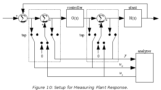
The entire system is shown in Figure 10. The block marked �analyzer� is implemented on the host, and communicates to the embedded processor via the communications link. The dotted boxes marked �tap� enclose the summing junctions and switches that connect one tap or another to the analyzer. The block marked �controller� is the controller being developed, and the block marked �plant� is the system being controlled.

5.1 Code

Assuming that there is a communications link, the additional software consists of three parts: the host-based stimulus generator, the embedded summing junctions, and the host-based results parser.

5.1.1 Embedded Code

Listing 1 shows the generic portion of the analyzer code that must be embedded in the system. This code depends on having three functions from the data interface: analyzerDataAvailable must return true if there is data to be read by analyzerGetInput; analyzerGetInput must return the latest stimulus data point sent by the host; and analyzerOutput must send the given output values to the host.

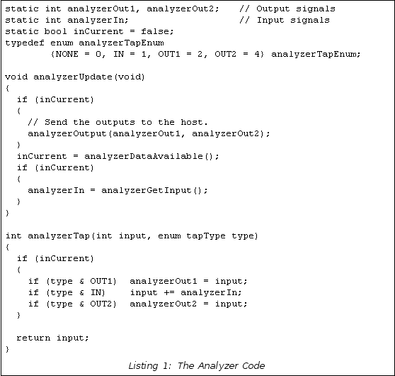
The function analyzerTap implements the taps shown in Figure 10. Depending on the value of the �type� input it will set the analyzerOut variables and inject the analizerIn signal into the summing junction. The function analyzerUpdate implements the interface between the host and the embedded system. It insures that there is data waiting, receives it, and sends the most recent collected analyzer data to the host.

Listing 2 shows how the analyzer code is used. The normal operation of this code is to get the ADC input, update the controller, and send the controller's drive command to the DAC. To implement the analyzer we insert the two calls to analyzerTap and the call to analyzerUpdate.

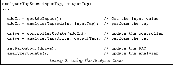
The values of the analyzer type inputs must be managed to insure that each analyzer signal is only connected to one tap. How the values of inputTap and outputTap are set determines the measurement that will be taken. For instance, to implement the plant transfer function measurement shown in Figure 3 you would set inputTap = OUT1 and outputTap = IN | OUT2; to implement the loop transfer function measurement shown in Figure 4 you would set inputTap = NONE and outputTap = IN | OUT1 | OUT2.

5.1.2 Host-Side Code

The embedded code doesn't have much functionality: it just shoves the signals around. In order to make the system work it is necessary to put most of the �brains� of the into the host side. The host side must generate the appropriate waveforms at the appropriate frequencies for the appropriate amount of time, and it must be able to receive the data, parse it, and show results.

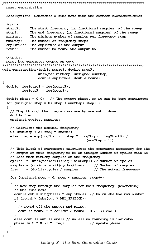
Listing 3 gives the code that generates the sine wave into standard output. It is presumed that this output will be piped to a file and sent to the embedded system using a terminal program or other means. The code generates a wave that is swept in frequency in a number of distinct segments, with the frequency varying logarithmically. The frequency of each segment and the segment length are calculated so the segment is an exact integer number of cycles long, with segments padded out in length as necessary to get a full cycle.

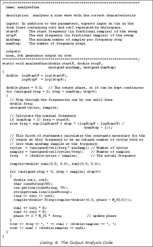
Listing 4 gives an example of the analysis code. Given the same set of parameters it generates the same frequency sequence as Listing 3, but in this case it reads in a line of system output at each sample step and performs demodulation described in (3) for each frequency step, then prints the result as text.

Of course, the code shown so far has a number of shortcomings that would need to be overcome in a real system: the Bode plot isn't actually printed, the format needed by Listing 4 is anonymous so the parameters must be remembered separately from the file, C++ isn't the best language for scientific computation of this sort, etc. All of these issues can and should be overcome in a real system, but these listings illustrate the point.

6 Other Methods

This subject is a small subset of the overall subject of system identification and control. Other popular methods of designing control systems for plants with unknown characteristics are the Ziegler-Nichols and Astrom-Hagglund methods for tuning PID controllers, ARMA system identification methods, and frequency response methods using random excitation. Each one of these methods has their advantages and adherents, and there are cases in control system design where one of these methods is clearly superior to the swept-frequency response measurement method shown here. I feel, however, that this method is the best overall method for tuning motion control loops in an embedded software environment. It has certainly served me well.

Tim Wescott, Z Transforms for the Embedded Engineer, http://www.wescottdesign.com/articles/zTransform/z-transforms.html

Peter A Cook, Nonlinear Dynamical Systems, Prentice-Hall International (UK), 1994.

Rick Lyons, Understanding Digital Signal Processing, 2^nd Edition, Prentice-Hall, 2004

HP 3563A Operating Manual � Control Systems Analyzer, Hewlett-Packard Company, 1990, HP Part number 03563­900000

HP 3563A Getting Started Guide � Control Systems Analyzer, Hewlett-Packard Company, 1990, HP Part Number 03563­90202