
Systems - Embedded Software - Circuits
by
(note: For a much more in-depth discussion of the z transform,
and other practical uses of control theory, see the book Applied Control
Theory for Embedded Systems.)
The z transform is an essential part of a structured control system design. This paper describes the basics of using the z transform to develop control systems, using the sort of math that is familiar to the accomplished embedded system designer.
1 Introduction
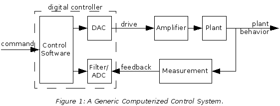
This paper talks about closed-loop (or feedback) control systems. This is the case when you are implementing a system like the one in Figure 1. The control software combines the feedback with the command to create the drive signal. The drive signal is amplified and applied to the plant, which changes its behavior. The plant behavior is measured and read by the control software as feedback. Since this all goes in one big circle it is called "closed loop".
The z transform is useful, but it only works on certain types of problems. If you can describe your plant and your controller using linear difference equations, and if the coefficients of the equations don't change from sample to sample, then your controller and plant are linear and shift-invariant, and you can use the z transform. If the problem at hand won't allow you to model the plant and controller as linear shift invariant systems you won't be able to use the z transform.
While all real-world plants are nonlinear in some sense, and have parameters that vary with time to some degree, the majority of plants can be usefully modeled with linear time invariant differential equations. Once this is done the effects of sampling the input and updating the output at discrete intervals can be taken into account and a difference equation that describes the plant behavior from the software's point of view can be produced.
Let's say that you've reduced the behavior of the plant to a difference equation that looks like
|
|
(1) |
where xn is the output of the plant at sample time n, un is the command to the DAC at sample time n, and the various a and b are constants set by the design of the plant, driver and ADC circuits.
You can solve (1) for xn over time if you are given a specific sequence of un using techniques very similar to those used to solve differential equations, but the process is just as tedious and obscure as solving differential equations, and just as error prone and frustrating. Furthermore if you want to investigate what happens when you add feedback to the system you would need to solve many equations like (1) over and over again. The z transform allows you to do both of these things.
2 The z Transform
Just as the Laplace transform is used to solve linear time-invariant differential equations and to deal with many common feedback control problems using continuous-time control, the z transform is used in sampled-time control to deal with linear shift-invariant difference equations.
Officially, the z transform takes a sequence of numbers xn and transforms it into an expression X(z) that depends on the variable z but not n. That's the transform part: the problem is transformed from one in the sampled time domain (n), and put it into the z domain. The z transform of x is denoted as Z(x) and defined as
|
|
(2) |
For example, if you have a signal xn = an you can plug it into (2) and get
|
|
(3) |
There are some complex rules about the values of z for which (2) is valid. While these rules are important in proving the mathematical solidity of the z transform they don't make much difference in it's practical application and can be safely ignored.
The most commonly used and most important property of the z transformation is that the z transform of a signal that is delayed by one sample time is the z transform of the original signal times z-1
|
|
(4) |
This seems pretty simplistic, but we'll get a lot of mileage out of it. Table 1 lists some other properties of the z transform (see [1]). If you feel inclined, it's good practice to use (2) or (4) to verify each one of these properties.
|
Property |
Comments |
|
|
|
k must be a constant. |
(5) |
|
|
(5) and (6) together imply that the z transform is a linear operation. |
(6) |
|
|
This is called a "first difference" -- it�s the discrete time equivalent to a differential |
(7) |
|
|
A summation is the discrete time equivalent to an integral. |
(8) |
|
|
This is the unit delay -- it's the fundamental operation in discrete-time analysis. |
(9) |
|
|
This is called the "Final Value Theorem" and is only valid if all the poles of X(z) are stable. |
(10) |
Table 1: z Transform Properties.
2.1 An Example
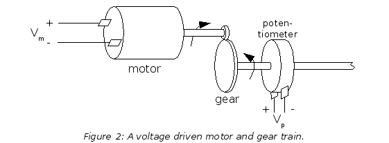
Figure 2 shows a motor and geartrain that we might use in a servo system. We're driving it with a voltage, and reading the position of the output gear with a potentiometer. Let's say that we're going to use it as our plant. If we ignore all the nonlinearities in the system, and any difficulties with the motor performance changing over time, and if we set x = vp and u = vi, then the difference equation that describes it might look like
|
|
(11) |
You can take the z transform of (11) without knowing what xn or un are by applying (2) as appropriate (remember that xn transforms to X(z) and un transforms to U(z)). If you do this you get
|
|
(12) |
Notice a cool thing: We've turned the difference equation into an algebraic equation! This one of the many things that makes the z transform so useful. It is perfectly fair to treat z as an algebraic variable. If we do so we can solve (12) easily [2]:
|
|
(13) |
|
|
(14) |
With (14) we have a general solution for (11), which applies for any input signal we may want to try out. If we know the z transform of u we can find the z transform of x very easily by plugging it into the right-hand side of (14). Then we could find the inverse z transform of the result to find out what x is in the time domain.
If this was all that we could do with the z transform it would be a useful tool to have around, but probably not something you'd want in your toolkit for everyday use. Fortunately, the z transform goes beyond allowing easy solutions to specific difference equations.
2.2 Transfer Functions
We can take the idea of plugging in signals one step further and express the relationship between X and U in (14) as a ratio:
|
|
(15) |
The function H(z) is called the "transfer function" of the system � it shows how the input signal is transformed into the output signal. In z domain terms the transfer function of a system is purely a property of the system: it isn't affected by the nature of the input signal, nor does it vary with time.
One easy and obvious thing that we can do with the transfer function in (15) is to predict the behavior of the motor. Let's say I want to see what the motor will do if x goes from 0 to 1 at time n = 0, and stays there forever. This is called the "unit step function", and a system's response to it is very informative. The z transform of the unit step response is z/(z-1). To simplify the math, lets also say that a = 0.8 and that b = 0.2. In that case I have
|
|
(16) |
and
|
|
(17) |
There's two ways I can go with (17). First, I can solve it by polynomial division. This is a good way to go if I want to graph the response vs. time, and it is simple to do. The result looks like this
|
|
(18) |
The system response is now expressed as a polynomial in z-1. It is trivial to apply (4) in reverse to get
|
|
(19) |
(19) gives the system response for that particular input. This is very useful, but you would like to know if the system will ever settle out, or what it will settle out to. The second method that you can use is partial fraction expansion to break things down into easy bits, followed by doing the reverse transform by inspection. The partial fraction expansion of X(z) is
|
|
(20) |
You can use (20) with the transforms in Table 2 to get
|
|
(21) |
When you do this it becomes immediately clear that the motor position and velocity start at zero, then the motor velocity increases with its velocity increasing asymptotically to one count per step. This is exactly what you'd expect from a motor with a constant voltage on it.
In fact, for all but a few special cases there will always be certain elements of the system response (in this case the 1 and the 0.8n) that will be there because of the nature of that system's transfer function. These special cases happen because the input signal happens to mask portions of the system output; in general this will not be the case.
|
|
|
Comments |
|
|
|
|
(22) | |
|
|
|
(23) | |
|
|
|
|
(24) |
|
|
|
|
(25) |
|
|
|
This is nasty, I haven�t found a better one yet. |
(26) |
|
|
|
a (and therefore b) must be a constant. |
(27) |
|
|
|
a (and therefore b) must be a constant. |
(28) |
|
|
|
a and b must both be constants, the pole is complex. |
(29) |
|
|
|
a and b must both be constants the pole is complex. |
(30) |
Table 2: Some common z Transforms.
2.3 Characteristic Polynomial
The derivation leading up to (21) points up a very important and useful property of the z transform: All of the elements in the response of the system to an input come from the system transfer function or from the input signal. Physically this happens because the system being modeled is linear. Mathematically this happens because the fractions that appear in a partial fraction expansion such as the one in (20) are the roots of the denominator polynomial of the output signal, which are in turn the roots of the denominator of the transfer function plus the roots of the denominator of the input signal.
What all this means is that the roots of a transfer function's denominator polynomial will nearly always make their presence known in the output of the system. This means that to get a general idea about how the system will behave you don't have to do all the work of putting a test signal into your system to see what comes out, you only need to factor the denominator and look at the value of its roots.
The usefulness of the transfer function denominator in predicting system behavior is so important, in fact, that control engineers refer to it as the system's �characteristic polynomial�. There is a whole lot of information just in the roots of the characteristic polynomial of a system, which are called the poles of the transfer function or system3.
The Fundamental Theorem of Algebra states that any polynomial can be factored into as many complex roots as the order of the polynomial4. Remember that a complex number is the sum of a real number and an imaginary number, such as 0.8 + i0.6, where i is the square root of �1. Remember also that a complex number can be expressed as a magnitude and a phase, so that 0.8 + i0.6 = 1.0 36.9.
When you raise a complex number by an integer, the magnitude of the result is the magnitude of the original number raised by the integer and the angle of the result is the angle of the original multiplied by the integer. This means that if I start with 0.99 10 and raise it to the 10th power the result is 0.9910 100, which is equal to about 0.90 100. Because of this property of complex numbers a system with poles of magnitude greater than one will "blow up": the system response will grow exponentially. System poles with magnitude close to one indicate a system that will settle slowly5.
3 Z Transforms and Software
One of the very nice things about the z transform is the ease with which you can write software from it. Since you'll be implementing controllers in software this is very important. You can do a theoretically correct job of coding from a transfer function almost by inspection. If you have a transfer function
|
|
(31) |
it turns into the z domain equation
|
|
(32) |
which can be converted by inspection into the difference equation
|
|
(33) |
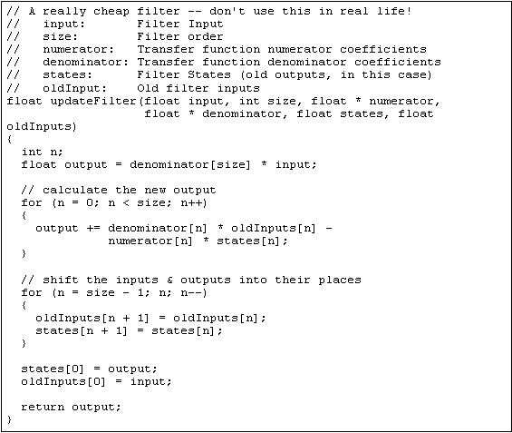
In turn this difference equation can be turned into software very quickly, as shown in Listing 1:
3.1 A Better Filter
The filter implemented in Listing 1 really isn't very good for a number of reasons. First, it uses floating point, which is quite slow on many embedded processors6 and can have problems with precision. Second, it uses more storage than is really necessary (in the "oldInputs" array).
Finally, and most important by far, is that Listing 1 implements a transfer function of unlimited order in one step. When a transfer function is implemented by the algorithm in Listing 1 the required precision rises rapidly with the order of the denominator polynomial. A guideline to use is that the precision of your math needs to be better than the precision of your input plus the precision required to accurately express each of the roots of the denominator.
As an example of this, if you have input from a 12-bit ADC that you want to run through a 2-pole low-pass filter with a double pole of 0.9 you would have a transfer function that would look like
|
|
(34) |
To maintain accuracy with the code in Listing 1 you would need at least 12 bits for the incoming data, plus 3.3 bits for each pole (to distinguish 0.9 from 1.0). Rounding up you need a bare minimum of 12 + 7 = 19 bits � and 24 would be even nicer. Keep in mind your pole position, however! If you need to filter down to a really low frequency, with a pole at 0.999, say, you'll need 10 bits per pole, for 12 + 20 = 32 bits. If you wanted to use a third-order filter, you'd need 43 bits � for data that's only good to 12 bits!
The way around this is to use the fact that any transfer function can be broken down into a cascade of 1st and 2nd order filters. This is the case because the transfer function of two filters in cascade (i.e. the output of one filter drives the input to the next) is equal to the product of the two transfer functions, so any transfer function can be factored into a number of cascaded ones. Any long transfer function should be broken up this way when this sort of filter is used (or a number of short transfer functions shouldn't be grouped, as the case may be).
If you stick to filters of no more than 2nd order, 32 bit words will work nicely on most processors for most filters with most sets of input data. Keep in mind that if you do have the luxury of using floating point that IEEE single precision floating point ("float" in most modern C and C++ compilers) only uses a 24 bit mantissa, which often isn't enough. Double precision floating point uses a 48-bit mantissa, which is much, much better, but double precision floating point will almost certainly be slower.
For some simple control problems you can often get by with 1st order filters and 16 bit words. This can be the case even if your input data is 16-bit, as long as the control doesn't have to be very fine when the difference between your feedback and it's target position need more than eight bits to express.
When you factor a transfer function you should factor it into 1st-order blocks whenever possible. For 2nd-order blocks I have a second-order filter that I like to use7 when I'm not coding for a DSP. It's a bit more complicated to analyze, so I'm just going to present it here. It starts with the difference equations
|
|
(35) |
If you work through the math you'll find that the resulting transfer function is
|
|
(36) |
The code is in Listing 2. This code gets rid of the need to store a separate state vector for the input, and unrolls the computation. You could rearrange this even more to get rid of the temporary state should you wish to give up some understandability for execution speed.
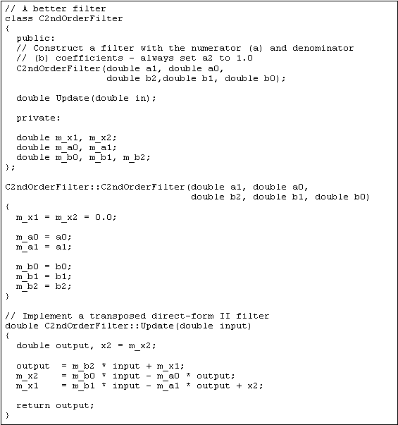
Listing 2: A Better Filter.
3.2 The PID Filter
What about the ubiquitous PID controller8? You could just use the filter in Listing 2, but PID controllers usually work better if you add limiting to your integrators, and a PID controller can be better coded as a differentiator in parallel with an integrator. Listing 3 shows a PID controller that has been written for the purpose. If you study the code and ignore the limiting9 you can write down the difference equation, then find the transfer function in the z domain.
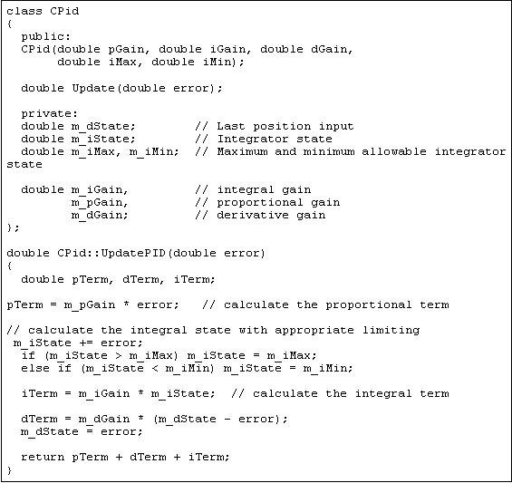
The difference equation looks like
|
|
(37) |
The z transform of this is
|
|
(38) |
Eliminating the state variables gives you
|
|
and finally,
|
|
In (39) you can see the effect of the three gains; in (40) you can see the transfer function of the filter.
4 The z Transform and Feedback
So how about using this in a control problem? Lets say that you want to use the controller described by (40) to control the plant described by (14). Control engineers like to reduce control systems to block diagrams like the one shown in Figure 3. This is an extremely simple system, which is reflected in the extremely simple diagram.

What Figure 3 shows is that the only input to the controller, e, is an error signal that is equal to the plant output, x, subtracted from the setpoint, u. This error signal drives the plant input, uc which in turn drives the plant output, closing the loop. We'd like to know, in general, how this system responds to inputs. Solving this problem using difference equations would be difficult and roundabout. Solving it with transfer functions in the z domain is straightforward.
I'll start by writing the expression for the plant output, x:
|
|
We know that we can get Uc(z) from E(z):
|
|
Now substitute (42) into (41) to get:
|
|
But e = u x! We can stick this relationship into (43) to get an equation in U and X:
|
|
(44) |
and solve for the transfer function of the system:
|
|
(45) is a classic equation in closed-loop control theory. Now we can go way back to (15) (for H) and (40) (for G) and stick them into (45) to get
|
|
(46) |
This "simplifies" to
|
|
|
|
|
If the system is sampled at 250Hz and the mechanical time constant of the motor with its load is 100 milliseconds then a = 0.96. This can be plugged into (48) to get
|
|
We can use (49) to predict what will happen to our system as well as to design systems.
With b set to 1 I built a simulation of the system shown in Figure 3 and adjusted the gains according to the method outlined in [3]. The gains came out to be kp = 0.5, ki = 0.1 and kd = 0.7. Then (49) becomes
|
|
This system has poles at z = 0.44 i0.37 and z = 0.78. These poles all have magnitudes that are much smaller than 1, so the system is not only stable, it settles fairly quickly.
5 The Frequency Domain and the Z Transform
So far in my presentation I've stuck to math, and we've found some results that are mathematically valid, but not really useful enough to write home about. The last section showed us how to take a system and describe it, but it didn't show how to use a system description to arrive at a result. (50) tells us that a hypothetical system is stable, but only if the real system matches the system that we've modeled - and we all know that our models don't always match reality! We also don't know anything about how well our system will fare as the parts age, or as multiple units are manufactured with differing component tolerances. Furthermore there isn't a really good way to go from real measurements of a system to a z domain model.
It is often very informative to excite a system with a unit sine wave input and look at its response. In the z domain exciting a system with transfer function H with a sine wave shows up mathematically as:
|
|
(51) |
If you do all the multiplying and the fractional expansions and whatnot you'll find that after all the transients due to the structure of H settle out yn is a sine wave with amplitude equal to |H(ejq)| and phase shift equal to H(ejq)10. These numbers are called the gain and phase of the system response (or the system gain and phase).
You can define the whole system's behavior using only its gain and phase response. In fact, you can do a whole closed-loop system design entirely with gain and phase responses, without ever needing a z-domain model of the plant. This works because there are some very useful things that you can do with gain and phase responses, not least of which is designing safe, stable control systems with well defined behavior. This means that if you don't have a good model of the system (or you suspect the model you have) you can take its real system frequency response and design a controller without ever needing to know its exact z transform.
Look back at Figure 3, and at (45). In a single-loop feedback control system, the overall transfer function will have a denominator that takes the form 1 + G1(z)G2(z) .... The value of G1(z)G2(z) ... is called the loop gain of the system, and can usually be identified by inspecting the block diagram of the system. Any value of z that causes the loop gain of the system to equal �1 will drive denominator to zero; by definition such a value of z is a pole of the system. This means that we can find out if we're close to a pole of the closed loop system by inspecting its open loop behavior.
Now assume that you've whomped up a closed loop system that is known to be stable. Further assume that you know the plant gain and phase response. You know that since the system is stable, the poles of the system must lie within the unit circle. Your job is to design a control system that keeps those poles in the unit circle while achieving your other design goals.
If the system parameters change in a continuous manner the system poles will move in a continuous manner. This means that any condition that will move a system pole to the unit circle will move the pole right out of the unit circle if it gets a bit worse. If you scan z around the unit circle while plotting gain and phase you can look for the places where the open loop gain is close to 1; these are the places where your stable poles may escape into the unstable region, so they are the places that you need to be concerned about. Such a gain-phase plot is called a Bode Plot.
5.1 Gain and Phase Margins
Traditionally the way that you express the robustness of a control system is by talking about its Gain Margin and Phase Margin. Both of these are measures of how close the open loop gain of the system is getting to 1. The idea is to determine the amount of plant variation you will see before the loop gain gets to �1 and the system goes unstable. The amount of gain change11 required to get you to �1 when your phase is 180 is the gain margin; the amount of phase change required to get you to �1 when your gain magnitude is 1 is the phase margin. Gain and phase margins of 6dB (a factor of two) and 60 is considered very safe, gain and phase margins of 3dB (square root of two) and 30 is pushing it.
So how does this work? For the PID example above, (14) and (40) give us the loop gain:
|
|
(52) |
You can scan z along the unit circle by using the relation 1 = cos() + isin() or 1 = ei. You'll want to use a math package that will handle complex numbers, such as MathCad, MatLab, Maple, etc. In a pinch you can whip up a display program in C or C++, but the graphing becomes a chore.
Figure 4 shows the gain and phase vs. angle12 of the loop gain for the controller with our example gains of kp = 0.5/b, ki = 0.1/b and kd = 0.7/b. The gain magnitude crosses 1 at = 1, where the phase is �150o, indicating a phase margin of 30o, and the gain phase crosses 180o at a magnitude of about 9 and 0.3 for gain margins of 19 and 10dB, respectively13.
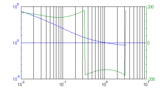
Figure 4: Gain/Phase plot of the motor & PID controller together.
The first thing to notice about this result is that the phase margin is a bit too small -- as I said previously, 30� is pushing it. Notice that this system appeared to be perfectly safe when we designed it using the traditional PID methods, and its poles were comfortably inside the unit circle, yet we've already found a potential problem! This indicates that if you just used the PID tuning method you could end up with a system that goes unstable when the temperature changes, or that was stable in the lab but doesn't always build to a stable system in production.
So how do we proceed? Let's look at our available tools for some clues. Figure 5 gives the Bode plot of the plant alone. Notice that the plant's phase approaches 180� pretty quickly. This is why we can't just wrap the motor with position feedback, unless we don't mind a low performance system. Figure 6 shows the Bode plot of the controller. See how the controller phase is positive for angular frequencies between about 0.4 radian/cycle and 3 radians/cycle? This extra phase makes the plant more stable.
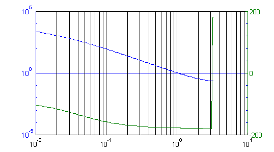
Figure 5: Gain/Phase plot of the plant alone.
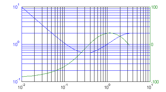
Figure 6: Gain/Phase plot of the PID controller.
Figure 7 shows the Bode plots of an integrator. Here you can see why an integrator decreases stability -- it's phase is essentially 90� for most useful frequencies. Since most systems need more positive phase rather than less, an integrator usually isn't the right thing to use for stability. So why use one? Look at the gain at low frequencies: the gain of the integrator goes to infinity as the frequency goes to 0. This means that the integrator will force the DC error of the system to zero, which is just another way of saying that it will insure that the system will always drive to the correct target.
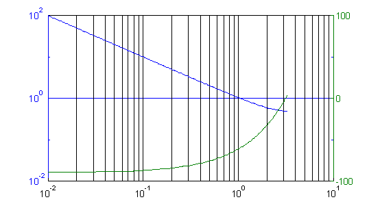
Figure 7: Gain/Phase plot of an integrator.
Figure 8 shows the Bode plot of the differentiator. The differentiator is just about the opposite of the integrator: while the integrator drives the phase negative and does good things at DC, the differentiator drives the phase more positive, which increases stability, but it doesn't do anything at DC, and it amplifies noise (which is bad).
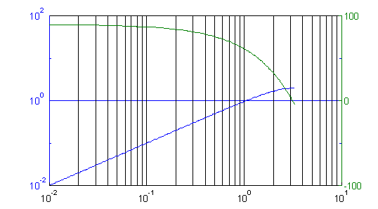
Figure 8: Gain/Phase plot of the differentiator.
As you can see from these plots, if we can increase the effect of the differentiator (or decrease the effect of the integrator and proportional term) we should see an increase in the phase margin of the system. I used this to tune the motor, Figure 9 shows the resulting open-loop bode plot with kp = 0.08/b, ki = 0.004/b and kd = 0.8/b. The gain margins are now 40dB and 7dB, and the phase margin is a nice comfortable 61o. What's more, the unity-gain frequency, which gives a rough measure of the system response speed, hasn't changed all that much, indicating that we've increased the stability of the system without losing too much performance.
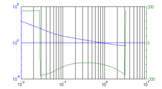
Figure 9: Open-loop gain with tuning.
5.2 Time-Domain Implications
Bode plots tell you all about system stability in the frequency domain, but they don't directly tell you if the system is going to meet its performance criteria, or how it will perform in the time domain. Unfortunately, we are usually not directly interested in the frequency domain performance of a system we're usually much more interested in what happens in the time domain. There really isn't a direct correspondence, but there are some generalities that can be made:
The settling time of the closed-loop system is roughly equal to the inverse of the bandwidth of the closed-loop response (usually measured from the frequency is 3dB or 6dB down from the DC value). Since the bandwidth of the loop response is strongly related to the unity gain frequency of the open loop response, this number can also be used.
If the closed-loop amplitude response rises from its DC value, the time domain response to a step input will likely overshoot. If the closed-loop amplitude response is "peaky", i.e. if it has a narrow rise of more than 3dB or so the step response will "ring". In fact, if the closed-loop amplitude response falls off sharply from its maximum gain the step response will ring. All of these conditions are caused by mild to extreme lack of phase or gain margin.
6 Finally
This paper has presented the very basics of control system design using the z transform. Using the z transform you can intelligently design stable, well behaved systems with performance that can be made predictable and reliable over variations in manufacturing tolerances and environmental conditions.
Bibliography
1: Constantine H. Houpis, Gary B. Lamont, Digital Control Systems, Theory, Hardware, Software, 1985
2: Gene H. Hostetter, Clement J. Savant, Jr., Raymond T. Stefani, Design of Feedback Control Systems, 1982
3: Tim Wescott, PID Without a PhD, , 2000
1 d(n) is the z transform equivalent of the Dirac delta function.
2 u(n) is known as the �unit step function�. Note that it is defined at n = 0
3 Because the magnitude of the transfer function as z varies over the complex plane goes to infinity at each denominator root, as if it were a circus tent with a pole right there.
4 Multiple roots must be counted individually, so z3�3z2+3z�1 has three roots at z = 1.
5 "Close to one" and "slowly" vary with the problem at hand, of course�
6Although some DSP chips can do floating point nearly as quickly as they can do integer arithmetic. This property is not common.
7 This is not the usual biquad filter, but it does essentially the same thing and I think it makes for tighter code on a general purpose processor.
8 See [3].
9 This is an example of linearization, where you're taking a non-linear system and modeling it as a linear one.
10 x is the angle that x makes to the real number line, it is equal to the arctangent of the imaginary part of x and the real part of x.
11 In decibels (dB). A gain in dB is equal to 20 times the logarithm to the base 10 of the linear gain: gaindB = 20log10(gainlinear).
12 The angle of z on the complex plane is related to frequency by the sampling time T. When z = ej it implies that the response will have a component ejn, which is a sinusoid with a frequency of /T radians per second, or /(2T) Hz.
13 Yes, you can have more than one gain or phase margin, because there's more than one gain or phase crossing or you can have no gain or phase margin.
Copyright 2004, Tim Wescott, All Rights Reserved.
 .
.  .
. .
. .
. ;
; .
. .
. .
.